When it comes to designing complex geometric shapes and forms, Grasshopper is an incredibly powerful tool that can help you achieve your goals. However, in order to make the most of this program, you need to have a solid understanding of some of the key concepts that underpin its operation. One of these concepts is the idea of parametric curves, which are curves that are defined by a set of parameters. In this blog post, I’ll take a closer look at how parametric curves work in Grasshopper, as well as the importance of curve parameters and domains.
Table of Contents
1. Parametric Curves in Grasshopper
To begin with, let’s define what we mean by a parametric curve. Simply put, a parametric curve is a curve that is defined by a set of parameters, rather than by a fixed set of points. In Grasshopper, these parameters are typically represented by variables that can be manipulated to create a wide range of different shapes and forms. One of the key benefits of using parametric curves is that they allow for greater flexibility and precision in designs, as it can be easily adjust by parameters to achieve the desired outcome.
From the mathematical point of view:
A parametric curve is a curve that is defined by a set of equations that specify its coordinates as functions of one or more parameters. For example, a 2D parametric curve can be defined by the equations x(t) and y(t), where t is the parameter. The curve is then represented by the set of points (x(t), y(t)) for all values of t.
2. Non-uniform Parameterization
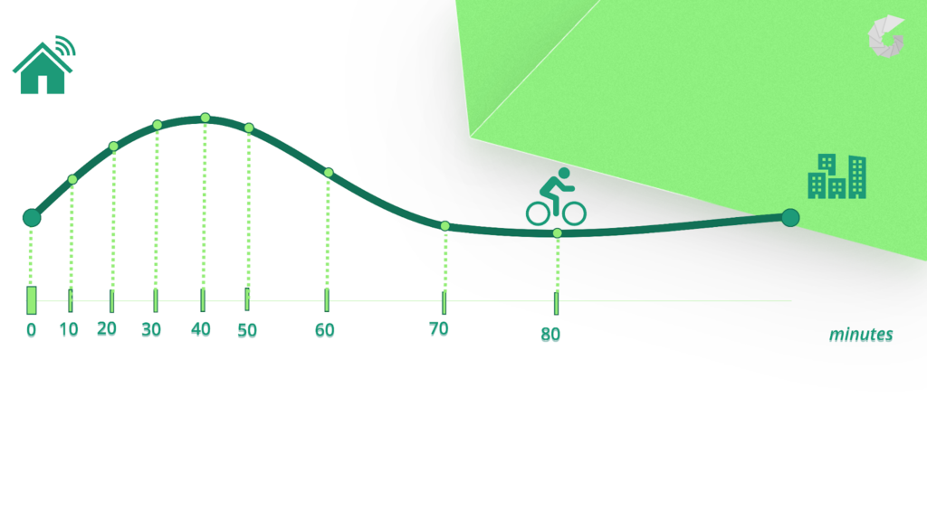
To better understand these concepts, let’s consider an example of Bob travelling from his house to the city on his bicycle. Bob’s path can be represented as a parametric curve, and the points at which he stops to check his progress can be considered as control points. Bob wears a watch to keep track of time and always checks how long it takes him to get to the city and measure his positions every 10 minutes. This journey can be represented as a parametric curve.
To create this curve, we can use the points where Bob checked the time as control points. These points help define the curve’s shape and direction. We can say that the time is our parameter in this case.
Bob checked his time every 10 minutes, which means we can use those points as our control points. This type of parameterization is called non-uniform, where the distance between control points defines how steep the slope is.
A non-uniform parameterization of a curve is one in which the parameter values are not evenly spaced along the curve. Non-uniform parameterizations can be useful in situations where we want to emphasize certain parts of the curve or achieve certain visual effects. We notice that the distance between each control point is not equal. For example, Bob had to cycle uphill, which took him more time than when he cycled downhill. This difference in time affects the distance between each control point.
The parameterization helps us understand the curve’s behaviour and how it changes as we move along it.
3. Uniform Parameterization
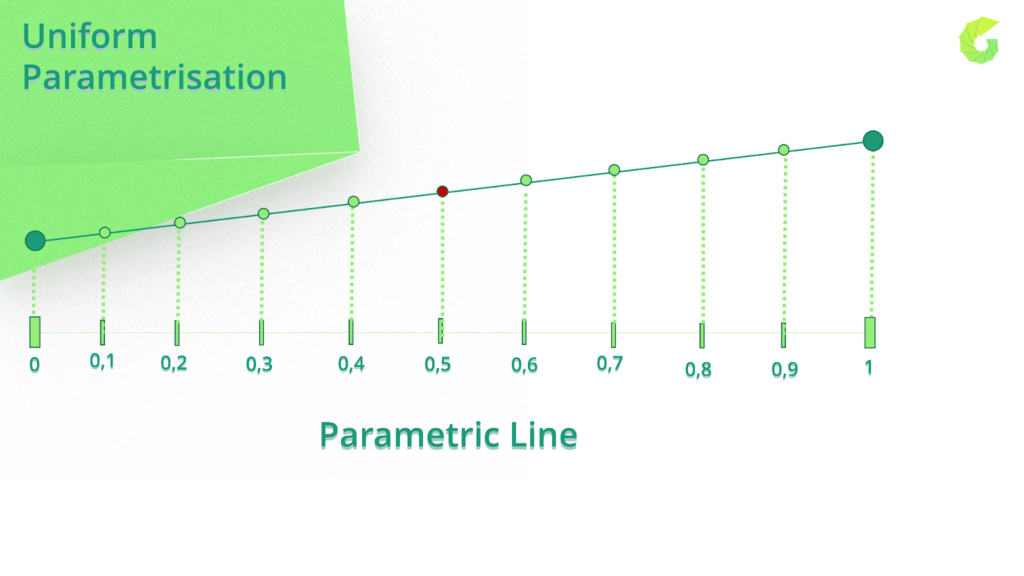
Let’s say that Bob is now travelling with the constant speed to the another city on a road that has a constant slope, meaning that he doesn’t have to ride uphill and downhill. In this case, we can use a Uniform curve Parameterization for the parametric curve that represents Bob’s journey.
With a Uniform curve Parameterization, we would divide Bob’s journey into equal intervals of time. Let’s say we divide his journey into 10 intervals of 10 minutes each. At the end of each interval, we would record Bob’s position along the road, just like we did with the non-uniform parameterization.
Since the slope of the road is constant, the distance Bob travels during each interval is also constant. Therefore, the distance between each control point along the parametric curve would be equal. This is what we mean by uniform curve parameterization.
A uniform parameterization of a curve is one in which the parameter is evenly spaced along the curve. This means that the distance between two adjacent parameter values is constant. A uniform parameterization can simplify many operations on curves, such as computing the length of the curve or interpolating points on the curve.
4. Parametric Curve Domain
Ok. So that was simplified explanation of non-uniform and uniform control point distribution on a parametric curve. Now lets go to another important topic.
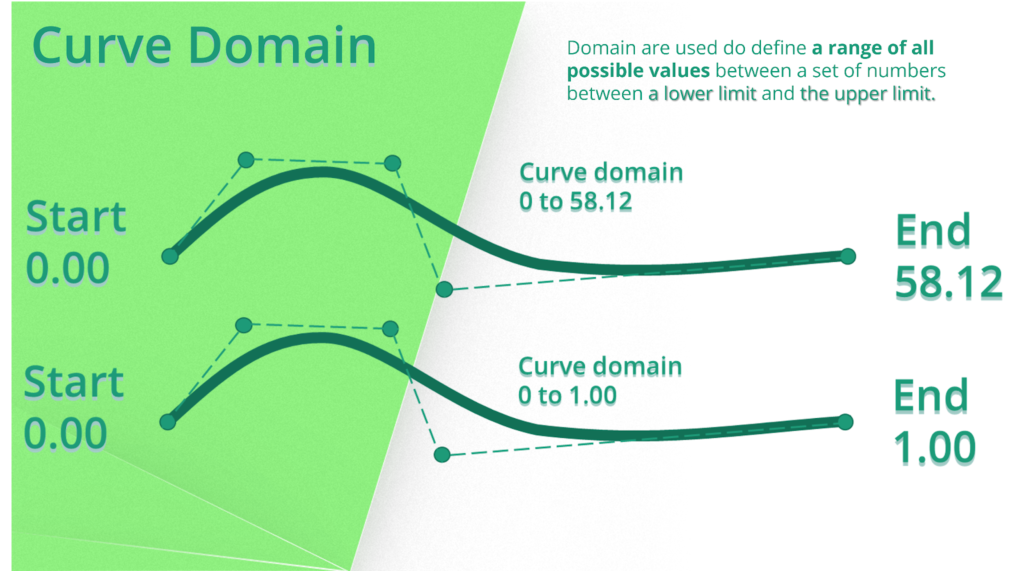
In Grasshopper, a curve’s domain is the range of values that correspond to the parameterization of the curve. Essentially, the domain is a set of numbers that define how the curve is parameterized, or how its points are ordered along the curve.
Lets take Bob bicycle ride to the city with the constant slope. In this example we have a simple curve like a line, its domain might be defined as 0 to 1. This means that if we evaluate the curve at a parameter value of 0, we will get the first point on the curve, and if we evaluate it at a parameter value of 1, we will get the last point on the curve.
In the first Bob bicycle ride on the non-uniform curve, the domain was more complex and variable compared to uniform curves. When Bob started his watch it measured his position (start) with the parameter equal to 0 on the curve. Then every single second we could track Bob’s position on the curve. Until the 120 minutes when he finished his trip. That’s why the domain of this parametric curve was from 0 to 120. Parameter 120 shows the end of the curve.
The domain of a non-uniform curve is defined by its control points, and the distribution of the control points along the curve affects the shape of the curve. The domain is a set of values that represents the range of parameters used to define the curve.
In Grasshopper, we can use various components to work with the domain of a curve. For example, we can use the “Curve Domain” component to retrieve the domain of a curve.
5. Reparameterize
As I wrote before, in Grasshopper, you can change the domain of a curve to whatever numbers you like. This process is called parameterization. However, it is strongly recommended that you stick to the default domain of 0 to 1 when using the Reparameterize component. This is because the 0 to 1 domain is a standard representation that allows you to work with curves in a consistent and predictable manner. Of course, unless you have a specific reason to do otherwise and change the domain to your needs.
Reparameterization in Grasshopper can be done in different ways:
Reparameterize component – All you need to do is connect your curve to the input of the component, and set the desired domain that you want to reparameterize to. The output of the component will be a new curve that has been reparameterized to the desired domain.
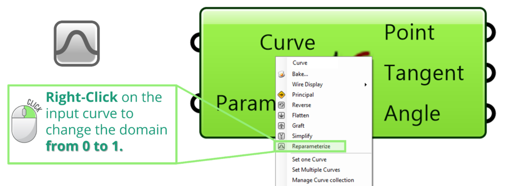
By setting the option on the Curve input or output. If there is any input or output with the curve text, you will see an additional sign of a parabola which means that for just one click, you can change the domain from 0 to 1.
6. Evaluate Curve Component
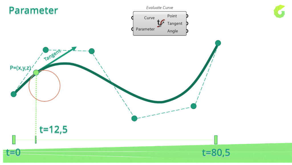
The Evaluate Curve component in Grasshopper is a tool that allows you to extract information from a curve at a specific parameter value. In other words, you can use this component to find out where a point on a curve is located or what the tangent direction of the curve is at a specific point.
To use the Evaluate Curve component, you need to provide it with a curve to evaluate and a parameter value at which to evaluate the curve. The parameter value represents a position on the curve, ranging from 0 to 1 in the default domain. You can also use the Reparameterize component to adjust the domain of the curve to better suit your needs.
Once you have provided the curve and parameter value to the Evaluate Curve component, it will output a point and a tangent vector corresponding to that position on the curve. You can use these outputs in various ways, such as to place an object at that point on the curve or to orient an object in the direction of the tangent vector.
7. Important aspect of parametric curves
When we measure a point at 0.5 on the parametric curve, it is not always in the middle of the curve in terms of total length. This is in contrast to uniform parameterization, where the distance between control points is equal, and the points are evenly distributed along the curve.
8. Summary
In this article, I explained the concept of parametric curves in Grasshopper, which are curves defined by a set of parameters rather than by a fixed set of points. Understanding domains and what the reparameterization process does to a domain. It is crucial to grasp the idea of parametric curves and start working with more advanced geometries.
